Topological Data Analysis and Persistent Homology

Posted on 26 Apr 2018

What is Topological Data Analysis?

Topological data analysis $\text{(TDA)}$ is a relatively new area of study in mathematics that takes abstract ideas and constructions from the branch of topology and applies them to data analysis. These novel approaches have led to interesting applications, and are worth having in your tool belt as a data scientist.

In this post, we will explore one construction that has come from TDA: persistent homology. We will give an overview of the construction of homology for simplicial complexes, and then show how that can be used for data analysis.

What is Topology?

Topology is a large branch of mathematics, and it studies the structure of spaces. Things that fall under the study of topology include the study of smooth manifolds, chaotic dynamic systems, and fractals. Applications of topology have a wide range, including protein folding, differential equations, chaos theory, theoretical physics, and data science. Some examples of topological spaces shown below

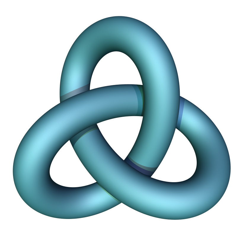
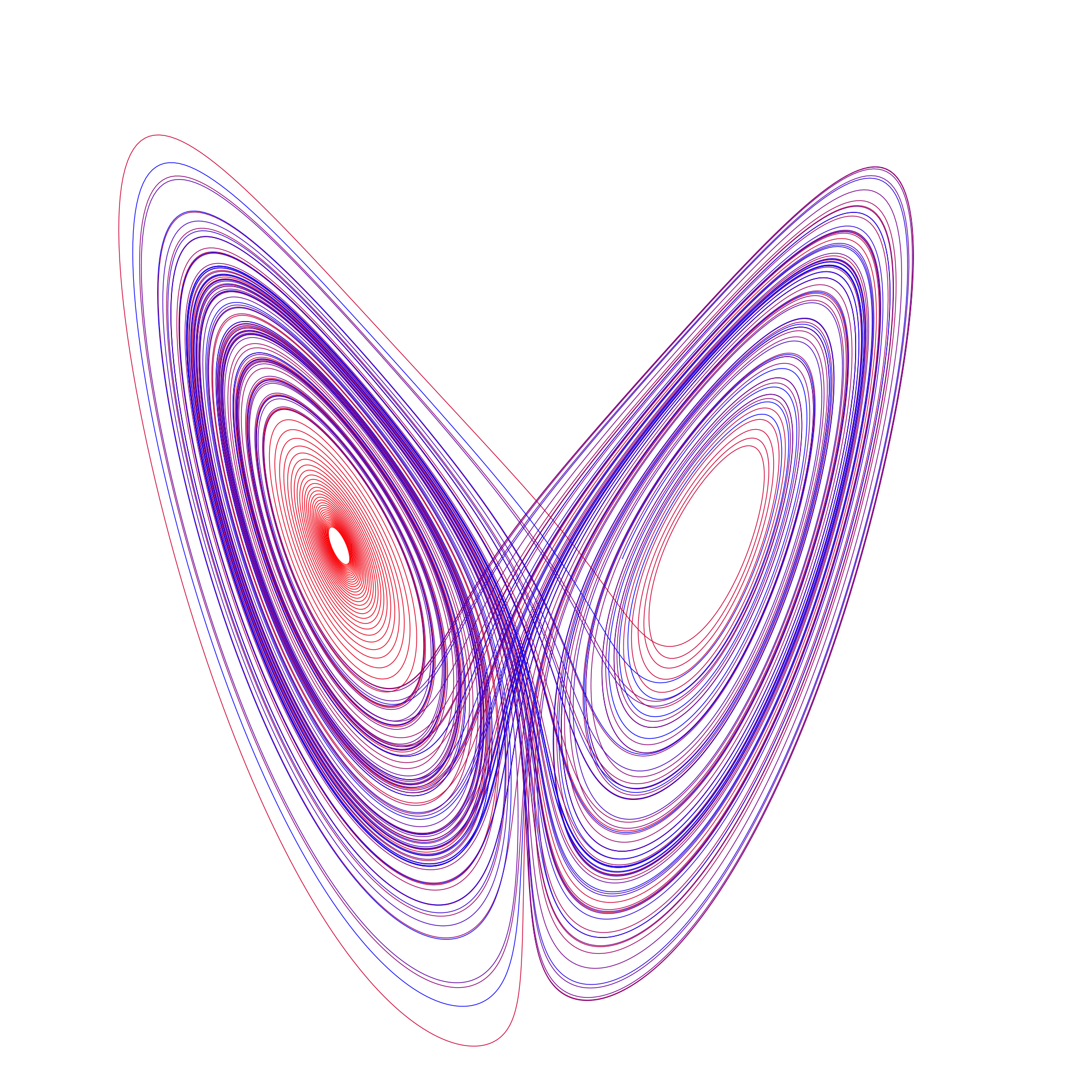
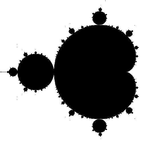
Above is the sphere, trefoil knot, Lorenz attractor and Mandelbrot set.

The sub-field of topology from with TDA was born is called Algebraic Topology. Algebraic topology views two spaces as being “the same” if they can be continuously deformed from one to the other. As illustrated by this gif, an algebraic topologist can’t tell the difference between a coffee cup and a donut!

Now, typically, deformations between spaces are very difficult to study directly. And in particular to show directly that two spaces are not the same up to a continuous deformation, you would need to show that there are absolutely no continuous deformations taking one space to the other. So instead, certain properties of spaces, that can be derived algebraically, and that respect deformations are studied. One of these properties is called homology.

Homology

Homology is an algebraic object constructed from a topological space that respects deformations in the sense that if two spaces can be continuously deformed from one to another, they will have identical homology. Intuitively, homology counts the “n-dimensional holes” in a space. One immediate application of homology is to be able to use it to tell two spaces apart: if their homology differs at all, then they cannot be the same.

Homology can be constructed for any topological space, but the construction is, in general, unwieldy. To get around this, we will restrict our attention to a nice class of spaces called simplicial complexes. These are simple enough to behave nicely, but complex enough to capture a wide range of spaces. We will explore these spaces next.

Simplicial complexes

A simplicial complex can be thought of as a generalization of a triangle or tetrahedron to arbitrary (positive) dimensions. In this post, we will be dealing with abstract, oriented simplicial complexes. Simplicial complexes are spaces that will be constructed out of simple building blocks called simplexes. Briefly, the 0-simplex is a point, the 1-simplex is a line connecting two 0-simplexes, a 2-simplex is triangle that has edges three 1-simplexes and vertices 0-simplexes, and so on.

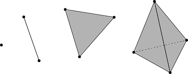
These building blocks will be used to construct simplicial complexes in general.

An abstract, oriented simplicial complex is a collection (S) of finite nonempty subsets of ({1, 2,…,n}) for some (n) such that if (A) is an element of (S), then so is every nonempty subset of (A). For example, the following are two simplicial complexes; a triangle with no interior, and a triangle with interior, and their graphical representations:

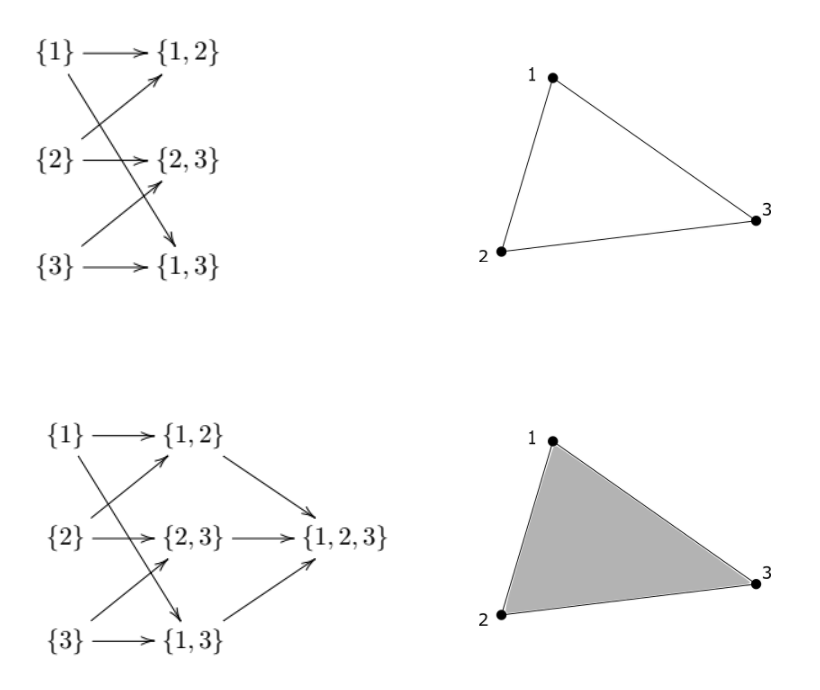
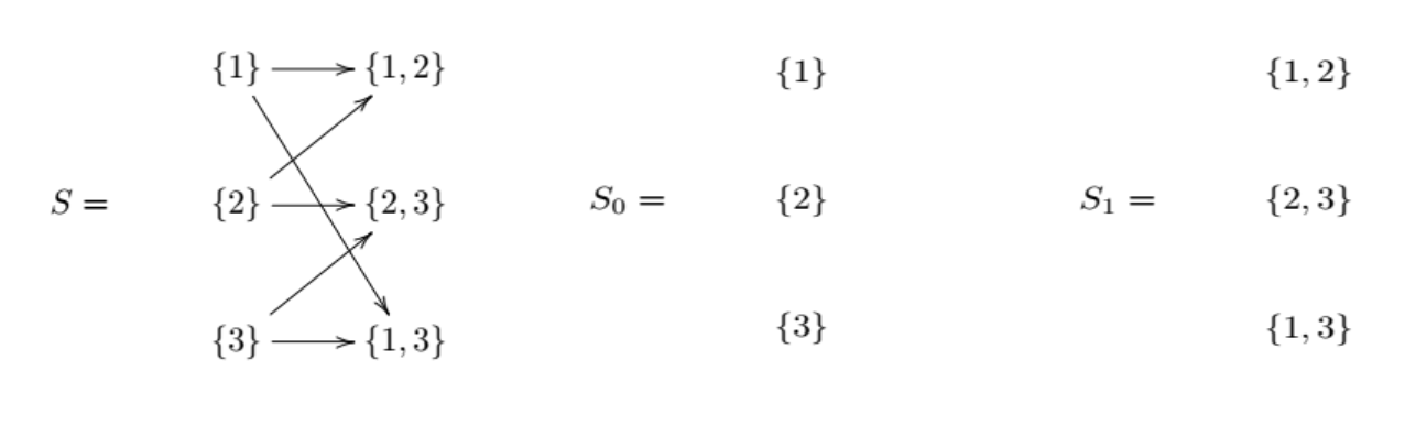
The one-element sets of a simplicial complex define it’s vertices (0-simplexes), the two-element sets define which vertices are connected by a line (2-simplex), and so on. Formally, for a simplicial complex (S), and an integer (k \geq 0), denote by (S_k) the collection of all sets in (S) with exactly (k+1) elements. We call (S_k) the (k-simplexes) of (S).

Next, we define the chain complex associated with a simplicial complex. Denote by (C_k) the collection of all finite linear combinations of elements of (S_k) with coefficients in the integers. We call (C_k) the (k-chains) of (S).

For example, (3\cdot{1, 2} + 1\cdot{2, 3} - 7\cdot{1, 3} ) is an element of (C_1).

For those not familiar with it, this construction is using a formal linear combination: there is no reduction to be done to the expression ( {1, 2} + {3, 4} ); it is simply a new element in the set (C_1 ). For intuition, we can think of ( C_k ) as being analogous to a vector space, and the elements of (S_k ) are the basis vectors for ( C_k).

Roughly speaking, a (k-chain) is a finite collection of (k)-simplexes, potentially with duplicates, and orientation. The 1-simplex ( {1, 2 } ) is thought of as having positive orientation going from the 0-simplex ({1}) to the 0-simplex ({2}). The element ( -{1, 2} ) of ( C_1) is thought of as the 1-simplex having orientation going from the 0-simplex ({2}) to the 0-simplex ({1}).

An example of adding elements in $C_1$ is

$$ \big(3\cdot\{1, 2\} + 1\cdot\{2, 3\} - 7\cdot\{1, 3\}\big) + \big(-4\cdot\{1, 2\} + 7\cdot\{1, 3\}\big) = -1\cdot\{1, 2\} + 1\cdot\{2, 3\}. $$

Boundary maps

There are maps ( \partial_k: C_k \rightarrow C_{k-1} ) called boundary maps. (\partial_k) is the ( \textit{k-boundary map} ).

(\partial_k) sends the (k)-simplex (\sigma = {\sigma_0, \sigma_1,…,\sigma_k} \hspace{3pt}) to

$$ \partial_k(\sigma) = \sum_{i=0}^k(-1)^i\{\sigma_0,...,\sigma_{i-1}, \sigma_{i+1},...,\sigma_k\}. $$

For example, $ \partial_2\big(\{1, 2, 3\}\big) = \{2, 3\} - \{1, 3\} + \{1, 2\} $.

These boundary maps give us the chain complex

$$ \cdots \xrightarrow{\partial_{k+1}} C_k \xrightarrow{\partial_k} C_{k-1} \xrightarrow{\partial_{k-1}} C_{k-2} \xrightarrow{\partial_{k-2}} \cdots \xrightarrow{\partial_3} C_2 \xrightarrow{\partial_2} C_1 \xrightarrow{\partial_1} C_0 \xrightarrow{\partial_0} 0 $$

An important relation between these boundary maps is that

\[\partial_{k-1} \circ \partial_k = 0\]

We will touch more on this in a bit. For a little illumination on why this is true, we give an example:

$$ \begin{align*} \partial_1\Big(\partial_2\big(\{1, 2, 3\}\big)\Big) &= \partial_1\big(\{2, 3\} - \{1, 3\} + \{1, 2\}\big) \\ &= \partial_1\big(\{2, 3\}\big) - \partial_1\big(\{1, 3\}\big) + \partial_1\big(\{1, 2\}\big) \\ & = \{3\} - \{2\} - \big(\{3\} - \{1\}\big) + \{2\} - \{1\} \\ & = 0 \end{align*} $$

The elements of the image of (\partial_k) in (C_{k-1}), denoted by (Im(\partial_k)), are called boundaries. These are simply the elements of ( C_{k-1} ) that arise as the boundary of an element of (C_k ).

All elements of (C_k) that are mapped to zero in (C_{k-1}) by (\partial_k) are called cycles. The cycles in (C_k) are denoted by (Ker(\partial_k)); i.e. cycles are elements of the kernel of (\partial_k).

We can now rephrase the above relation (\partial_{k-1} \circ \partial_k = 0 ) as $Im(\partial_k) \subseteq Ker(\partial_{k-1})$. In fact, for those familiar, (Im(\partial_k)) is a normal subgroup of (Ker(\partial_{k-1})), and (Ker(\partial_{k-1})) is a subgroup of (C_k).

If we take the following simplicial complex

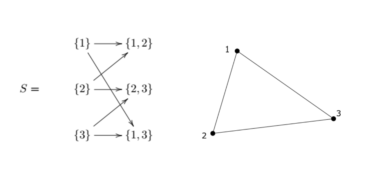
We can see that $\big( {1, 2} + {2, 3} - {1, 3}\big)$ is an example of a (k)-cycle that is not a (k)-boundary. It is a (k)-cycle because

$$ \partial_1\big(\{1, 2\} + \{2, 3\} - \{1, 3\}\big) = \{2\} - \{1\} + \{3\} - \{2\} - \big(\{3\} - \{1\}\big) = 0 $$

But it is not a (k)-boundary because there are no 2-simplexes in (S).

Homology

The (k^{th}) homology group of (S) is defined to be

\[H_k(S) = Ker(\partial_k) / Im(\partial_{k+1})\]

Informally, (H_k(S)) is “the (k)-cycles of (S) up to a boundary of a (k+1)-chain”.

For those familiar with group theory, the above definition of (H_k(S)) is the group (Ker(\partial_k)) quotient by the normal subgroup (Im(\partial_{k+1})). For those not familiar; this is saying that the (k^{th}) homology group is (Ker(\partial_k)) –all k-cycles, except that we treat all the elements of (Im(\partial_{k+1})) in it as zero. Recall that $Im(\partial_k) \subseteq Ker(\partial_{k-1})$. This is analogous to modular arithmetic; if we are doing arithmetic modulo 5, we are treating 5 the same as 0. So 6 = 5+1 (\equiv) 1 (mod 5). We will see some examples now.

Examples

Our first example is one to show that the (0^{th}) homology group, (H_0) counts the number of connected components of a simplicial complex.

$$ \cdots \xrightarrow{\partial_2} C_1 \xrightarrow{\partial_1} \color{#449CED}{C_0} \xrightarrow{\partial_0} 0 \\[20pt] $$ $$ \begin{multline} \shoveleft \begin{aligned} &C_0 = \mathbb{Z}\langle \{1\}, \{2\}, \{3\} \rangle \hspace{30pt} && Ker\partial_0 = C_0 \hspace{30pt} & H_0 = Ker\partial_0 / Im\partial_1 \\ &C_1 = \mathbb{Z} \langle \{1, 2\} \rangle \hspace{30pt} && Ker\partial_1 = \langle \{2\} - \{1\} \rangle \end{aligned} \end{multline} $$ $$ \begin{multline} \shoveleft \begin{aligned} & \{1\} = \{2\} - [\{2\} - \{1\}] = \{2\} - \partial_1(\{1, 2\})\\ & \text{So } \{1\} \equiv \{2\} \text{ in } H_0 \\ & H_0 = \mathbb{Z} \langle \{1\} \rangle \times \mathbb{Z}\langle \{2 \} \rangle \equiv \mathbb{Z} \times \mathbb{Z} \end{aligned} \end{multline} $$

The number of copies of (\mathbb{Z}) in (H_0) is the number of connected components of the simplicial complex.
The second example is one to show that the (1^{st}) homology group, (H_1), counts the number of 1-dimensional holes in the space.

$$ \cdots \xrightarrow{\partial_3} C_2 \xrightarrow{\partial_2} \color{#449CED}{C_1} \xrightarrow{\partial_1} C_0 \xrightarrow{\partial_0} 0 \\[20pt] $$ $$ \begin{multline} \shoveleft \begin{aligned} & C_0 = \mathbb{Z}\langle \{1\}, \{2\}, \{3\} \rangle \hspace{30pt} && Ker\partial_0 = \mathbb{Z}\langle \{1, 2\} + \{2, 3\} - \{1, 3\} \rangle \hspace{30pt} \\ & C_1 = \mathbb{Z} \langle \{1, 2\}, \{1, 3\}, \{2, 3\} \rangle \hspace{30pt} && Im\partial_2 = 0 \\ & C_2 = 0 \hspace{30pt} \end{aligned} \end{multline} $$ $$ \begin{multline} \shoveleft \begin{aligned} &H_0 \equiv \mathbb{Z} \\ &H_1 = Ker\partial_1/Im\partial_2 \equiv \mathbb{Z} \end{aligned} \end{multline} $$

The number of copies of $\mathbb{Z}$ in (H_1) is the number of 1-dimensional holes in the space.
Our third example is one to demonstrate a bit more how boundaries are treated as zero in the homology group.

$$ \cdots \xrightarrow{\partial_3} C_2 \xrightarrow{\partial_2} \color{#449CED}{C_1} \xrightarrow{\partial_1} C_0 \xrightarrow{\partial_0} 0 \\[20pt] $$ $$ \begin{multline} \shoveleft \begin{aligned} & C_0 = \mathbb{Z}\langle \{1\}, \{2\}, \{3\}, \{4\} \rangle \hspace{30pt} \\ & C_1 = \mathbb{Z} \langle \{1, 2\}, \{1, 3\}, \{2, 3\}, \{2, 3\}, \{3, 4\} \rangle \hspace{30pt}\\ & C_2 = \mathbb{Z} \langle \{2, 3, 4\} \rangle \hspace{30pt} \end{aligned} \end{multline} $$ $$ \begin{multline} \shoveleft \begin{aligned} &Ker\partial_1 = \mathbb{Z} \big\langle \left[\{1, 2\} + \{2, 3\} - \{1, 3\}\right], \hspace{5pt} \left[\{2, 3\} + \{3, 4\} - \{2, 4\}\right] \big\rangle \\ &Im\partial_2 = \mathbb{Z} \langle \{3, 4\} - \{2, 4\} + \{2, 3\} \rangle \\ &H_1 = Ker\partial_1/Im\partial_2 \equiv \mathbb{Z} \langle \{1, 2\} + \{2, 3\} - \{1, 3\} \rangle \end{aligned} \end{multline} $$

Since the element ({3, 4} - {2, 4} + {2, 3}) is treated as zero in (H_1), we have that (H_1) is generated by all the other elements of (Ker\partial_1), namely the element ({1, 2} + {2, 3} - {1, 3}). Thus (H_1) has only one copy of (\mathbb{Z}).

Topological Data Analysis

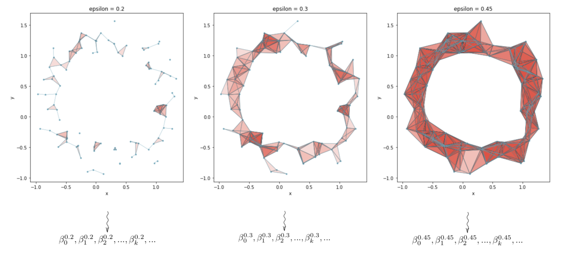
One branch of TDA takes a dataset in (\mathbb{R}^n), typically called a point cloud, and associates to it a sequence of simplicial complexes. We then find the homology groups of each simplicial complex in this sequence, and analyze this sequence of homology groups. One of these simplicial complexes in this sequence is formed by first viewing all the points as the 0-simplexes in the simplicial complex. Then we choose a number (\epsilon > 0), and connect any two 0-simplexes with a 1-simplex if the two points are less than distance (\epsilon) apart. Then we connect 2-simplexes onto this space wherever there is a triple of 0-simplexes, all of which are less than distance (\epsilon) apart from one another. The higher dimensional simplexes are added similarly. We formalize that a bit now.

Let (X) be our data set/point cloud. For each (\epsilon > 0), we construct a simplicial complex (S) as follows. Let

\[S^{\epsilon}_0 = \big\{ \{p\} : p \in X \big\}\]

and

$$ S^{\epsilon}_k = \big\{ \{p_1, p_2,..., p_{k+1}\} \mid p_i \in X \hspace{4pt} \text{and} \hspace{4pt} |p_i - p_j| < \epsilon \hspace{4pt} \text{for every} \hspace{4pt} i, j \big\}. $$

Then we set

\[S^{\epsilon} = \bigcup S^{\epsilon}_k.\]

The colletion ({S^{\epsilon} \mid \epsilon > 0}) is called the Vietoris-Rips filtration, or sometimes just the Rips filtration.

Below is a depiction of three simplicial complexes formed from the same point cloud for three different choices of (\epsilon), as well as a cartoon of the homology groups being calculated for each simplicial complex.

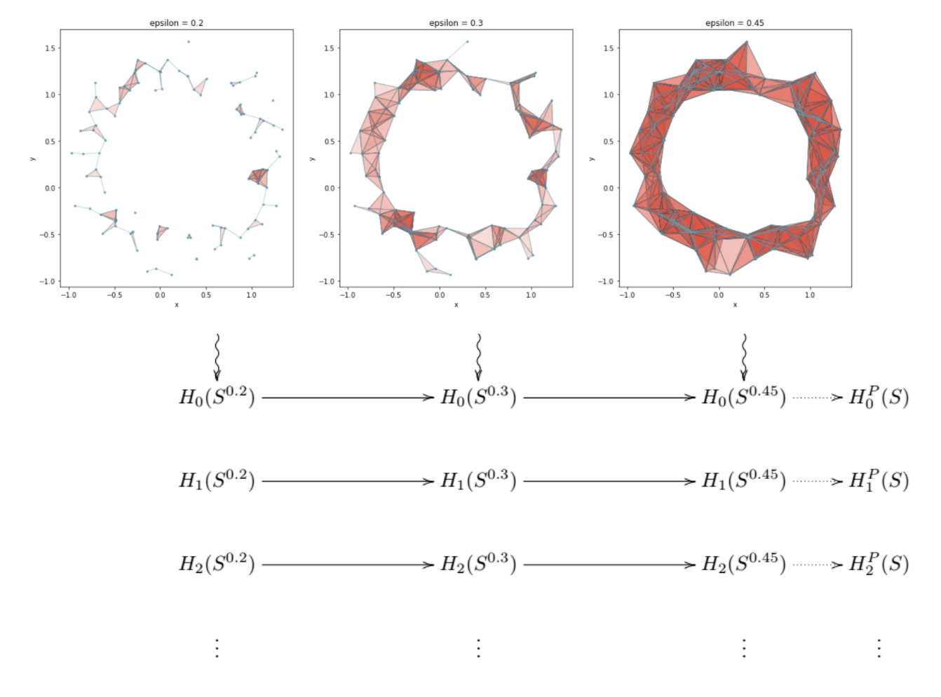
To the far right of the grid of homology groups, there are depicted groups $H_0^P(S), H_1^P(S), …$. These are the persistent homology groups. This post is a bit of a misnomer, as we will not be defining or going into great detail about the actual persistent homology groups. Instead, we will focus more on Betti numbers, which are derived from the persistent homology groups, and are more useful to data scientists.

Barcodes and Persistence Diagrams

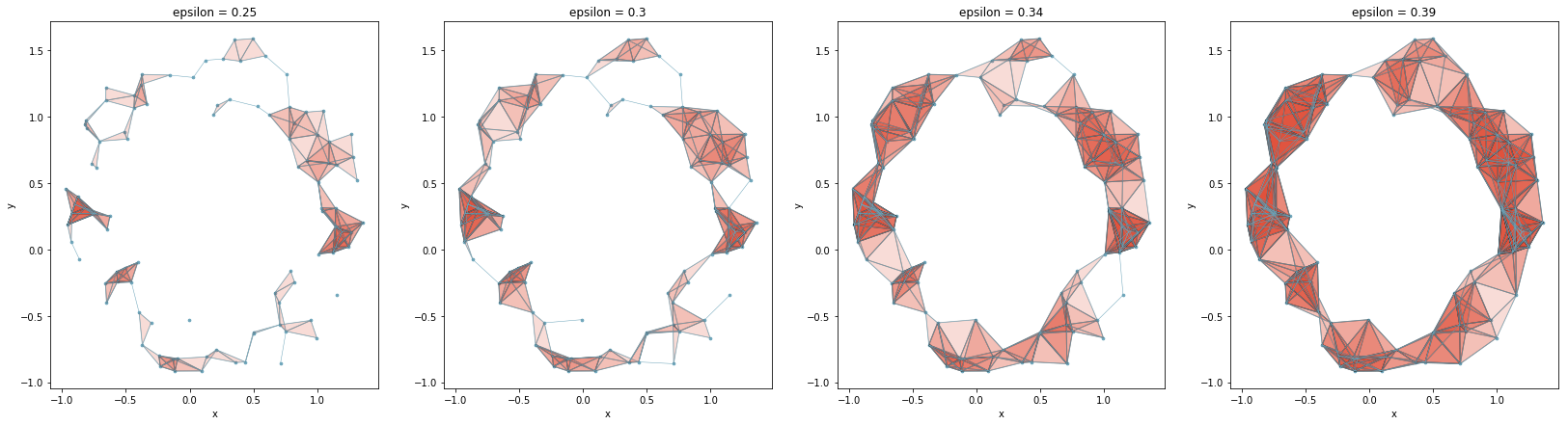
Before we dive into Betti numbers, we will discuss two common methods of visualizing persistence data: the barcode diagram and the persistence diagram. In the image below, we have four simplicial complexes for a point cloud for epsilon values of 0.25, 0.3, 0.34, and 0.39. We can see that as epsilon becomes larger, 1-dimensional holes in the space are formed. These holes will exist for a range of epsilon values, until epsilon becomes large enough to “fill in” the hole. That is, each of these holes persist for an interval of epsilon values. The holes that persist the longest are the ones that we think of as being a feature inherent to the data, whereas the shorter ones are seen more as noise in the data. In this example, there is one hole that seems to be inherent in the data, and the others are noise.

To encode the data of how long holes are persisting for in this sequence of simplicial complexes, the barcode diagram is typically used. Below is the barcode diagram for the above point cloud

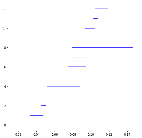
Each horizontal line represents a hole in the data, and the length tells us how long it persists. For example, a horizontal line whose left endpoint has x-coordinate 0.05, and right endpoint has x-coordinate 0.10 means that there was a nonzero element in (H_1(S_{0.05})), and it persisted through (H_1(S_{0.10})), at which point it disappeared. The left and right x-coordinates of one of these horizontal lines are called the birth point and death point respectively. For our example the birth point would be 0.05, and the death point would be 0.10.

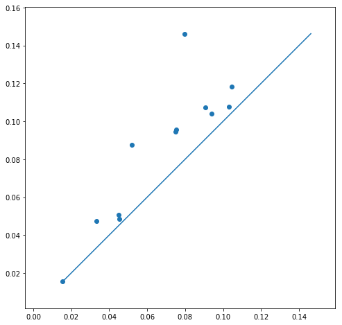
Another way to visualize this persistence data is through what is called the persistence diagram. This is constructed by taking all (birth point, death point) pairs from the persistence diagram and plot them as x- and y- coordinates. A hole in the data that persisted for a very short time would lie very close to the (y = x) line, whereas one that persisted for longer would lie farther away. Below is the persistence diagram for the above point cloud

Betti numbers

The (k^{th} \textit{Betti number}) of a simplicial complex (S) is the rank of the (k^{th}) homology group, $H_k(S)$, and is denoted by (\beta_k). For intuition, if $H_k(S)$ were a vector space, the analogous quantity to the Betti number would be the dimension of the vector space; i.e. the number of basis vectors in a basis for the vector space. We can revise our image to

In the depiction above, note that (0 \leq k < 2).

We can then arrange the Betti numbers in a matrix form with dimensions (n_{\epsilon}\times d), where (n_{\epsilon}) is the number of choices for epsilon. In practice, we have to choose a finite set of (\epsilon) to use when building the Rips filtration. And (d) is the dimension of the data. In these depictions, (d = 2).

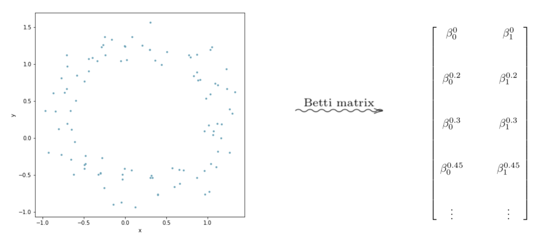
Graphing the columns of this matrix as line plots can lead to interesting interpretable results.

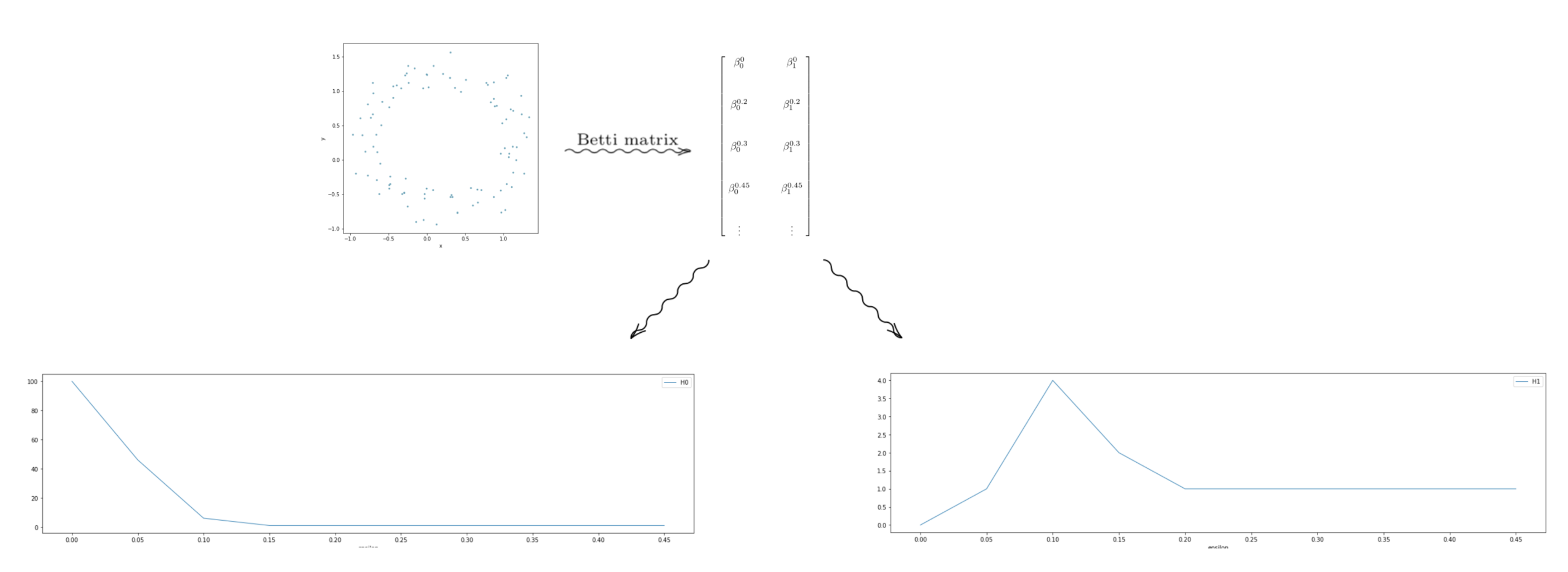
The point cloud depicted above looks roughly like a circle–but it has some “noise” in the data. But intuitively, we would say the data looks like it has one component, with a “hole” in the center of it. In terms of homology, we should have (H_0 \equiv \mathbb{Z}), and (H_1 \equiv \mathbb{Z}). Looking at the graphs, we see that the graph on the left, which is the Betti numbers of all the (0^{th}) homology groups starts high and levels out at 1. Thus, for most of the values of (\epsilon), the Betti numbers tell us that the space formed by the point cloud has one component. So we would conclude–pretending we don’t know what our data set looks like– that our data set is laid out in a single general component. Now looking at the graph on the right, we see that it levels out at 1. Through similar reasoning using Betti numbers, we can reasonably conclude that our data is laid out in a way that has a single 1-dimensional “hole” in it.

Hopefully now we have a better idea behind homology, persistent homology, and Betti numbers, and how they are constructed. In a later post, we will explore some applications of these ideas.

Image credits

Sphere: https://www.wikiwand.com/en/Sphere
Trefiol knot: https://theinnerframe.wordpress.com/tag/trefoil-knot/
Mug-torus gif: https://www.wikiwand.com/en/Topology
Lorenz attractor: https://commons.wikimedia.org/wiki/File:Lorenz_attractor.svg
Mandelbrot set: https://www.cs.princeton.edu/~wayne/mandel/mandel.html