Spectral Clustering
by Eric Bunch
Posted on 01 Jun 2018
Introduction
Spectral clustering is a way to cluster data that has a number of benefits and applications. It relies on the eigenvalue decomposition of a matrix, which is a useful factorization theorem in matrix theory. We will look into the eigengap heuristic, which give guidelines on how many clusters to choose, as well as an example using breast cancer proteome data.
Graph Clustering Method
Spectral clustering should really be viewed as a graph clustering algorithm, in the sense that a data clustering problem is first translated to a graph clustering problem, graph clusters are found, and then translated back to the data clustering problem. Spectral clustering gives a way of grouping together nodes in a graph that are similarly connected.
Pros & Cons
Here is a short list of some pros and cons of spectral clustering compared to other clustering methods.
Pros
- Clusters not assumed to be any certain shape/distribution, in contrast to e.g. k-means. This means the spectral clustering algorithm can perform well with a wide variety of shapes of data.
- Do not necessarily need the actual data set, just similarity/distance matrix, or even just Laplacian
- Because of this, we can cluster one dimensional data as a result of this; other algos that can do this are k-medoids and heirarchical clustering.
Cons
- Need to choose the number of clusters $k$, although there is a heuristic to help choose
- Can be costly to compute, although there are algorithms and frameworks to help
Speak here about importance of assumptions of kmeans clustering.
Eigenvalue Decomposition
For a square $n\times n$ matrix $M$, with $n$ linearly independent eigenvectors, we can find a factorization of $M$ as
\[M = UDU^{-1}\]Where $D$ is the diagonal matrix of eigenvalues of $M$. The $i^{th}$ column of $U$, ${\bf u_i}$ is the eigenvector corresponding to the $d_{i,i}$ entry of $D$.
Adjacency Matrix and Laplacian
In order to formulate the spectral clustering algorithm, we need to translate the data into a graph representation. Our aim will be to form the Laplacian matrix of the graph, and then perform spectral clustering on that. To do this we need a few objects:
- Graph representation of the data
- Degree matrix of the graph
- Adjacency matrix of the graph
Representing the Data as a Graph
There are a number of meaningful ways to represent a data set as a graph, and the most appropriate one to choose will of course depend on the particular data set and problem being addressed. We’ll outline a few standard methods here to get us started.
Similarity Graphs
In the following three similarity graphs, the set of nodes of the graph is defined to be the set of data points in the data set; denote them by ${v_1,…,v_n }$.
-
$\epsilon$-neighborhood Graph Here real number $\epsilon$ is fixed, and all nodes that are less than $\epsilon$ in distance apart are connected with an edge. This graph is typically considered as an unweighted graph.
-
$k$-nearest Neighbor Graph Here we place an edge between $v_i$ and $v_j$ if $v_j$ is among the $k$ nearest neighbors of $v_i$ or if $v_i$ is among the $k$ nearest neighbors of $v_j$.
-
Mutual $k$-nearest neighbor graph Here we place an edge between $v_i$ and $v_j$ if $v_j$ is among the $k$ nearest neighbors of $v_i$ and if $v_i$ is among the $k$ nearest neighbors of $v_j$.
Degree, Adjacency, and Laplacian Matrices of the Graph
For these definitions, we’ll think in general terms of a graph, and then come back to our special case. So let $G = (V, E)$ be an undirected graph with vertex set $V = {v_1,…,v_n}$.
Degree Matrix
The degree matrix $D$ of a graph $G = (V, E)$ is the $\mid V\mid \times \mid V\mid$ matrix defined by
\[D_{i,j} := \begin{cases} deg(v_i) & \text{if} \hspace{5pt} i = j \\ 0 & \text{otherwise} \end{cases}\]where $deg(v_i)$ of a vertex $v_i \in V$ is the number of edges that terminate at $v_i$.
Adjacency Matrix
The adjacency matrix $A$ of a simple graph–no edges starting and ending at the same vertex–$G = (V, E)$ the adjacency matrix is the $\mid V\mid \times \mid V\mid$ matrix defined by
\[A_{i,j} := \begin{cases} 1 & \text{if there is an edge between } v_i \text{ and } v_j \\ 0 & \text{otherwise} \end{cases}\]Notice that since we assumed $G$ was a simple graph, the diagonal entries of $A$ are all zero.
Lapacian Matrix
The Laplacian matrix $L$ of a simple graph $G$ is defined as
\[L = D - A.\]Stated differently,
\[L_{i, j} = \begin{cases} deg(v_i) & \text{if } i = j \\ -1 & \text{if } i eq j \text{ there is an edge between } v_i \text{ and } v_j\\ 0 & \text{otherwise} \end{cases}\]Normalized Laplacian
The normalized Laplacian matrix $L_{norm}$ of a simple graph $G$ is defined to be
\[L_{norm} := D^{-1}L = I - D^{-1}W\]Algorithm
Input: Similarity matrix $S \in \mathbb{R}^{n×n}$, number $k$ of clusters to construct.
- Construct a similarity graph by one of the ways described above. Let $W$ be its weighted adjacency matrix.
- Compute the normalized Laplacian $L_{norm}$.
- Compute the first $k$ eigenvectors $u_1,…, u_k$ of $L_{norm}$.
- Let $U \in \mathbb{R}^{n×k}$ be the matrix containing the vectors $u_1,…, u_k$ as columns.
- For ${i = 1,…, n}$, let $y_i \in \mathbb{R}^k$ be the vector corresponding to the $i^{th}$ row of $U$.
- Cluster the points $(y_i)_{i=1,…,n} $ in $\mathbb{R}^k$ with the $k$-means algorithm into clusters $C_1,…, C_k$. Output: Clusters $A_1,…, A_k$ with $A_i = {j| y_j ∈ C_i}$.
Example
In this section we will use spectral clustering on a manufactured data set from Scikit-learn; the noisy moons:
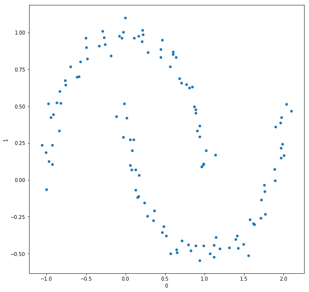
I chose to generate this data set to have 120 points, and a noise factor of 0.05. Below is a representation of the epsilon graph of this data set with $\epsilon = 0.1$.
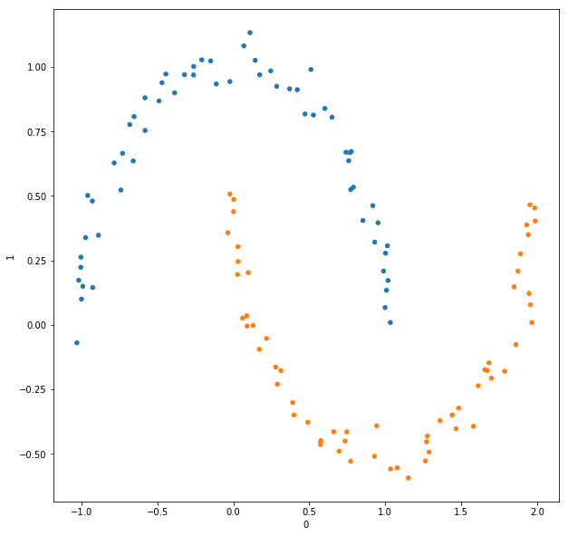
As we can see from the plot of the data as well as the graph visualization, there are two distinct clusters represented. We then compute the normalized graph Laplacian matrix $L_{norm}$, and find the eigenvalue decomposition it; that is, we find an invertible matrix $U$ and diagonal matrix $D$ where
\[L_{norm} = UDU^{-1}\]Since we are able to see the data, we can “cheat” and say we want to cluster the data into two clusters. In general, it is not possible to look at data and tell so easily how many clusters we should have. But there is a heuristic to help us choose the number of clusters, which we will learn about in the next section.
Since we have already determined that we are looking for two clusters, we take the two columns, ${\bf u_1}$ and ${\bf u_2}$, of $U$ corresponding to the two smallest eigenvalues of $L_{norm}$. Then we use $k$-means clustering with $k=2$ to obtain two clusters within the reduced data set $[{\bf u_1}, {\bf u_2}]$. We then “pull back” the cluster labels from $[{\bf u_1}, {\bf u_2}]$ to $U$, to $L_{norm}$, and finally to the data set. Labeling the clusters with different colors, we can see the graph depiction is colored as expected
And if we plot the original data set with the clusters marked with different colors, we get an expected picture.
How to Choose $k$: Eigengap Heuristic
With spectral clustering, there is a way to choose the number of clusters $k$ (of course it is not a hard rule, but a heuristic to help inform you). If we let $\lambda_1,…,\lambda_n$ be the eigenvalues of the Laplacian, the goal is to choose $k$ such that $\lambda_1,…,\lambda_k$ are relatively small, but $\lambda_{k+1}$ is relatively large. Unfortunately, it does not seem so far like there is a simple, single-number metric that can be used to evaluate what number of clusters should be chosen.
Example: Breast Cancer Proteomes
In this example we look at breast cancer proteome data. This data can be found on Kaggle, and contains the proteome profiles for 77 breast cancer samples. After some preprocessing, a sample of the data looks like this:
| NP_057427 | NP_002408 | NP_000415 | NP_000413 | NP_000517 | NP_004439 | NP_005219 | NP_058519 | NP_058518 | NP_001116539 | NP_061155 | NP_001035932 | NP_077006 | NP_000917 | NP_065178 | NP_006836 | NP_006614 | NP_001784 | NP_006092 | NP_001153651 | NP_001159403 | NP_000116 | NP_004314 | NP_060601 | NP_005931 | NP_003003 | NP_113611 | NP_002002 | NP_004487 | NP_008950 | NP_114172 | NP_001062 | NP_001444 | NP_057547 | NP_054895 | NP_001246 | NP_055606 | NP_036451 | NP_000624 | NP_569082 | NP_001159 | NP_001229 | NP_002458 | |
|---|---|---|---|---|---|---|---|---|---|---|---|---|---|---|---|---|---|---|---|---|---|---|---|---|---|---|---|---|---|---|---|---|---|---|---|---|---|---|---|---|---|---|---|
| TCGA-A2-A0CM | 2.160157 | 2.623021 | 4.768355 | 0.639321 | 4.933663 | -4.419112 | -0.271711 | -6.013418 | -6.013418 | -6.318320 | 2.277710 | -4.029719 | -4.029719 | -6.509343 | 1.906685 | 2.215260 | -1.601524 | 1.631171 | 2.013217 | -6.395464 | 0.584219 | -4.937078 | -0.433346 | 3.126292 | -1.182743 | 0.286664 | 0.980958 | 1.509945 | -4.433806 | 2.549550 | 2.733226 | 0.896468 | 1.576068 | -1.292949 | 3.541400 | 3.177722 | 0.001309 | -1.792547 | -0.830502 | -0.538113 | 2.516489 | 2.556897 | -2.035927 |
| TCGA-A2-A0D2 | 2.249702 | 3.576941 | 2.169868 | 2.968207 | 0.543251 | -5.421010 | -1.206443 | -5.297932 | -5.277974 | -5.311238 | 2.934943 | -5.567372 | -5.567372 | -5.287953 | 1.198555 | 3.264258 | 2.449287 | 2.332862 | 3.606879 | -7.124134 | -0.853843 | -4.153646 | -2.417258 | -0.604362 | 2.545753 | 7.053044 | 2.921637 | 3.743262 | -6.269245 | 2.376105 | 2.781928 | 6.836827 | 2.898353 | -3.694601 | 2.495856 | 2.722053 | 0.373604 | -1.342826 | -4.183584 | -2.889608 | 3.487128 | 1.029442 | -0.714133 |
| TCGA-A2-A0EQ | -0.020957 | 1.884936 | -7.407249 | -7.675146 | -5.187535 | -2.795601 | 7.158672 | -9.114133 | -8.762041 | -9.573385 | -0.859091 | -1.241800 | -1.241800 | -7.047502 | 1.961478 | 0.863101 | 1.842838 | -0.369223 | 0.266075 | -3.055843 | -0.836128 | -6.308873 | -0.686872 | 0.162743 | -2.791774 | -5.554936 | 0.047930 | 3.388984 | 0.063239 | 0.545453 | -0.273546 | 1.460128 | -0.174083 | -1.410193 | 0.702364 | -1.402538 | 0.001309 | -0.210764 | 1.934688 | -0.538113 | 0.798041 | 2.003576 | -2.035927 |
| TCGA-A2-A0EV | -1.364604 | -2.246793 | -3.750716 | -3.882344 | -2.252395 | -3.252209 | -1.574649 | -2.190781 | -2.871327 | -2.190781 | -4.632905 | -2.608071 | -2.608071 | -1.266583 | 1.158737 | -2.039549 | -1.160160 | -1.216172 | -1.185366 | 0.466989 | -1.924724 | 0.649028 | -0.488016 | -6.134027 | 0.534203 | 1.080321 | -0.709263 | -1.199369 | -1.723081 | -2.179579 | -3.311022 | 0.139319 | 0.733046 | 0.018893 | -1.574649 | -4.515280 | 0.001309 | -0.210764 | 2.049328 | -0.538113 | -0.266769 | -3.201798 | -7.724769 |
| TCGA-A2-A0EX | -2.506723 | -2.953194 | -0.803378 | -2.315378 | -0.098028 | -1.643795 | -1.212331 | 4.186597 | 3.976493 | 3.942726 | -2.521730 | 0.427232 | 0.415977 | 1.545287 | 1.725376 | -1.812629 | -2.476708 | -0.923438 | -1.966455 | -2.037740 | -1.973959 | -2.409174 | 0.115828 | -0.882167 | 0.419729 | 1.031282 | -1.666306 | -0.083021 | -0.281869 | -3.752341 | -3.317125 | -2.769353 | -0.174083 | -0.822137 | -2.938187 | -3.395914 | -1.827636 | 0.082061 | 0.044543 | -2.079011 | -3.046991 | 2.554537 | -0.443199 |
We will go through this example twice: once with forming the epsilon graph from the data, and proceeding with spectral clustering, and another with forming the mutual nearest neighbors graph instead.
Epsilon Graph
Taking $\epsilon = 0.37$, we can form the epsilon graph from the data, and get the following graph
Next, we perform eigenvalue decomposition on the normalized Laplacian; $L_{norm} = UDU^{-1}$. We then plot the eigenvalues of $L_{norm}$ in increasing order
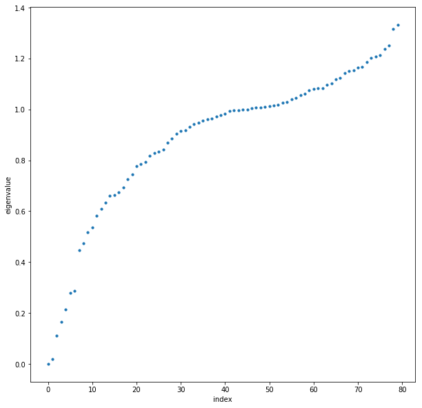
Using the eigenmap heuristic, we wish to choose an $n$ such that the first $n$ eigenvalues are relatively small, and $\mid \lambda_{n+1} - \lambda_n\mid$ is relatively large. It’s now up to our discretion what to choose, but looking at the eigenvalue plot as well as the network graph, I think it is reasonable to choose $n=4$. We then proceed with the spectral clustering algorithm: we choose the four eigenvectors in $U$ corresponding to the first four eigenvalues. Then we cluster on the lower dimensional data, and assign clusters to the original dataset accordingly. We show the graph representation of the data with clusters colored:
These are fairly decent clusterings, although it is a little “clumpy”: there are two main tightly connected clusters and a lot of nodes that are more loosely connected.
Mutual Neighbors Graph
Next, we look at the same proteome data set, but this time we will form the mutual neighbors graph during the spectral clustering process. With a little experimentation, we can find a good number of neighbors: here I chose 9 neighbors for the following graph. Already, we can see that this graph does not have the same “clumpy” look as the epsilon graph, and looks to have better clusters.
We perform the eigenvalue decomposition on the normalized Laplacian $L_{norm}$ and again plot the eigenvalues

Using the eigengap heuristic, let’s choose 5 clusters to cluster the data into. Then we proceed with the spectral clustering algorithm, and display the graph with the clusters colored.
These clusters look much better than those from the epsilon graph.
Conclusion
We have seen how spectral clustering works, and how it differs from other methods like $k$-means, as well as the eigengap heuristic and how it can be used to choose the number of clusters. The code to generate the examples in this post as can be found here.