Forecasting new home sales in the U.S.

Posted on 25 May 2017

In this post we will forecast the time series hsales, which can be found in the R package fma. The hsales data contains monthly sales of new one-family houses sold in the USA from 1973 to 1996. This analysis will be done in R using the forecast package.

Visualization and exploration

The time series plot hsales is below.

R> plot(hsales)

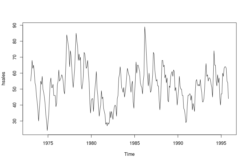
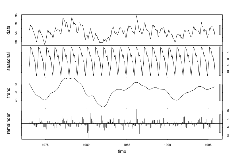
We can initially see that there is some seasonality in the data. Next, we plot the decomposition of the time series into seasonal, trend, and remainder components.

R> plot(stl(hsales, s.window="periodic"))

Transforming the time series

We will adjust the time series for seasonality by removing the seasonal component.


R> hadj <- seasadj(stl(hsales, s.window = "periodic"))
R> tsdisplay(hadj)

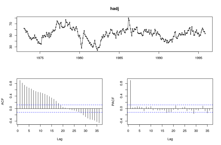
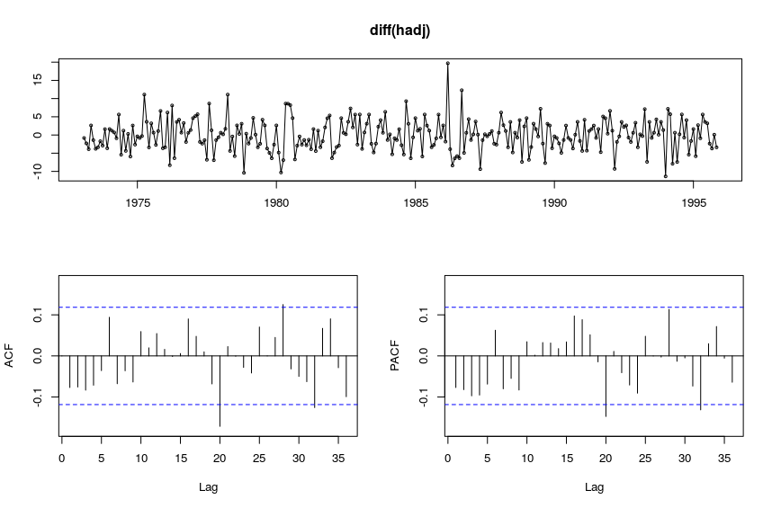
We will model the trend component (graphed above) of hsales. We will use a seasonal ARIMA model for this, which means we must transform the data into a stationary time series. The high PACF at lag 1 suggests we should difference the data with lag 1.

R> tsdisplay(diff(hadj))

We use the Augmented Dickey-Fuller Test to test for stationarity.


R> adf.test(diff(hadj))

Augmented Dickey-Fuller Test

data:  diff(hadj)
Dickey-Fuller = -7.4186, Lag order = 6, p-value = 0.01
alternative hypothesis: stationary

Warning message:
In adf.test(diff(hadj)) : p-value smaller than printed p-value

We can see that indeed, diff(hadj) is stationary.

Forecasting

The PCAF suggests that there are no large autocorrelations in diff(hadj), so we will first try ARIMA(1, 0, 0).


R> fit <- Arima(diff(hadj), order=c(1, 0, 0))
R> summary(fit)
Series: hadj
ARIMA(1,0,0) with non-zero mean

Coefficients:
         ar1     mean
      0.9013  52.5875
s.e.  0.0255   2.5165

sigma^2 estimated as 18.2:  log likelihood=-789.02
AIC=1584.04   AICc=1584.13   BIC=1594.89

Training set error measures:
                      ME     RMSE      MAE        MPE     MAPE      MASE        ACF1
Training set -0.05203778 4.251127 3.325061 -0.8537709 6.641165 0.4037355 -0.02679891

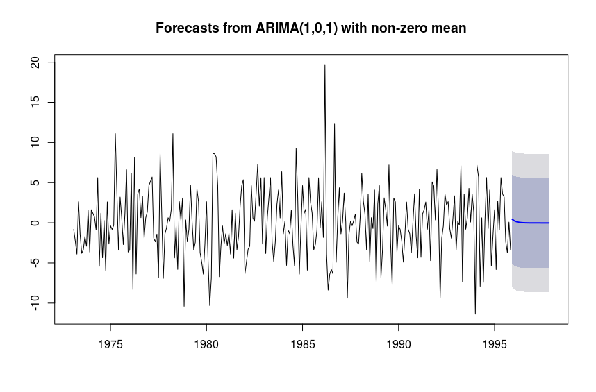
We also try other models close to the initial one chosen and compare AICc values to see which gives the lowest. Out of ARIMA(1, 0, 0), ARIMA(1, 1, 0), and ARIMA(1, 0, 1), the model with the lowest AICc is ARIMA(1, 0, 1), so we will choose this one.


R> fit <- Arima(diff(hadj), order=c(1, 0, 1))
R> summary(fit)
Series: diff(hadj)
ARIMA(1,0,1) with non-zero mean

Coefficients:
         ar1      ma1     mean
      0.6672  -0.7997  -0.0173
s.e.  0.1248   0.0984   0.1575

sigma^2 estimated as 18.65:  log likelihood=-788.17
AIC=1584.34   AICc=1584.48   BIC=1598.79

Training set error measures:
                     ME     RMSE      MAE      MPE     MAPE     MASE       ACF1
Training set -0.0149392 4.294922 3.360814 99.24458 115.8192 0.686308 0.02646853
R> plot(forecast(fit, h=24))

Testing residuals for white noise

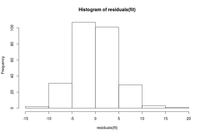
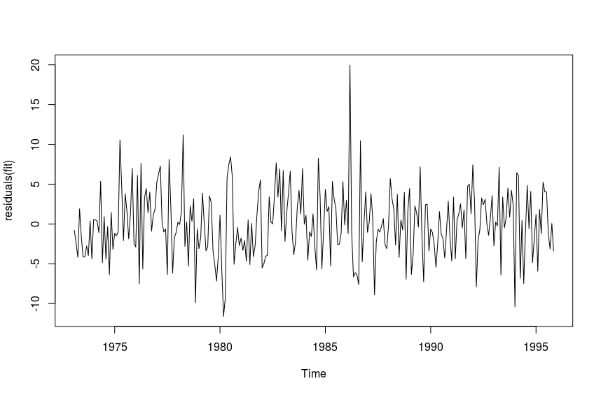
We need to test whether or not the residuals of the fit are white noise. We will plot the histogram of the residuals as well as the line plot first.

We will also use the Box-Ljung test to test if the residuals are white noise.


R> Box.test(residuals(fit), type = "Ljung")

  Box-Ljung test

data:  residuals(fit)
X-squared = 0.19407, df = 1, p-value = 0.6596

The p-value indicates that we can reject the null hypothesis, and assume the residuals are white noise. This means we have a decent fit to the time series, and we will proceed with reverse transforming the forecast.

Reverse transformation

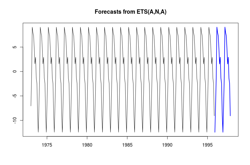
We have the forecast of the differenced, seasonally adjusted hsales time series. The transformations were not too outlandish, so the forecast interpretation is not terribly difficult, but we wish to reverse transform this forecast and plot it. To do that, we will first fit the seasonal part of hsales with a simple ETS model, and add this to the reverse transformed forecast of diff(hadj).


R> hseas <- stl(hsales, s.window="periodic")$time.series[,'seasonal']
R> sfit <- ets(hseas)
R> summary(sfit)
ETS(A,N,A)

Call:
 ets(y = hseas)

  Smoothing parameters:
    alpha = 0.0418
    gamma = 0.048

  Initial states:
    l = 0
    s=-12.4225 -9.0642 -2.4584 -1.3744 2.9153 1.5529
           4.7527 7.3438 7.9677 9.07 -1.2304 -7.0525

  sigma:  0

      AIC      AICc       BIC
-18629.63 -18627.78 -18575.38

Training set error measures:
                     ME        RMSE          MAE           MPE         MAPE MASE        ACF1
Training set 1.8571e-17 1.11224e-16 5.571301e-17 -4.056508e-15 4.056508e-15  Inf -0.02878259

R> plot(forecast(sfit, h=6))

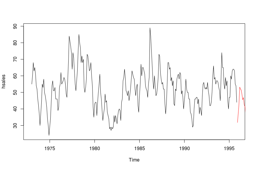
We then plot the original time series hsales as well as the transformed forecast for 24 months.


R> plot(hsales)
R> lines(diffinv(forecast(fit, h=24)$mean) + forecast(sfit, h=24)$mean + tail(hsales[-1], n=1), col='red')