Calculating Homology of a Simplicial Complex Using Smith Normal Form

by Eric Bunch

Posted on 24 May 2018

In this post, we will detail how to compute homology groups for a simplicial complex. Simplicial complexes are a nice subclass of topological spaces that are more easily described algebraically than general topological spaces. The notion behind homology is to algebraically compute the number of n-dimensional holes in the space.

Algebraic Topology

Algebraic topology is a sub-field of topology that is concerned with algebraic properties of spaces that respect homotopy. Briefly, a homotopy between two continuous functions $ f, g: X \rightarrow Y $ is a continuous function $H:X\times [0, 1] \rightarrow Y$ such that for all $x \in X$ we have $H(x, 0) = f(x)$ and $H(x, 1) = g(x)$. We think of $H$ as a continuous deformation of $f$ into $g$. We write $f \sim g$ to denote that $f$ and $g$ are homotopic.

Two topological spaces $X$ and $Y$ are homotopy equivalent if there are continuous functions $f: X \rightarrow Y$ and $g: Y \rightarrow X$ such that $f\circ g \sim id_Y$ and $g \circ f \sim id_X$.

Algebraic topology views two spaces as “the same” if they are homotopy equivalent. With this view then, it is interesting to ask: when are two spaces the same, when are they different, and are there ways to quantify how different two spaces are from each other? Now, studying homotopy equivalences directly is very difficult; for instance, to show two spaces are not homotopy equivalent, you need to show that there are absolutely no homotopy equivalences between the two spaces. And to show two spaces are homotopy equivalent you need to conjure up two continuous maps and two homotopies, and unfortunately there is no systematic way to construct this. Thus, a common method of attack for the types of questions posed above is to create algebraic invariants of spaces, and investigate those, linking them back to interesting properties of the spaces. The term invariant is used because we want these properties to be homotopy invariant; that is, if we construct a property $P$ for a space $X$, being homotopy invariant means that for any space $Y$ that is homotopy equivalent to $X$, the property $P$ for $Y$ is the same as the property $P$ for $X$. Homology is such a property. Homology also happens to have a nice intuitive explanation behind it as well. Unfortunately, homology is a bit cumbersome to define in total generality. So we will focus on a very common and useful class of topological spaces called simplicial complexes. These are spaces that are built out of simple components, and the homology can be much more easily computed.

Simplexes

Simplexes are the building blocks for simplicial complexes. Simplexes can be thought of a generalizations of a triangle to any non-negative integer dimension. The standard $k$-simplex (or just the $k$-simplex) is defined by the collection of points

Doing a quick sanity check, we can see that for $k = 0$, the $0$-simplex is the point ${1}$ in $\mathbb{R}$; for $k = 1$, the $1$-simplex is the line in $\mathbb{R^2}$ defined by $x_1 = 1 - x_0$; for $k = 2$, the $2$-simplex is defined by the $2$-dimensional plane $x_2 = 1 - x_1 - x_0$ in $\mathbb{R}^3$, restricted where each coordinate is positive; that is, it is a triangle. Generalizing this, we can see that the $k$-simplex is a $k$-dimensional subset of $\mathbb{R}^{k+1}$, and is the generalization of a 2-dimensional triangle in $\mathbb{R}^3$.

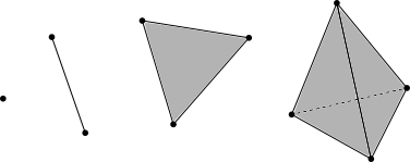
The faces of the $k$-simplex are the $k-1$-simplexes that make up its boundary. The boundary of the $k$-simplex (for $k > 0$) is the subset of the $k$-simplex where at least one of the coordinates $x_i$ is equal to $0$. The faces of the $1$-simplex are the two endpoints of the line segment; the faces of the $2$-simplex are the three $1$-simplexes of its boundary, and so on.

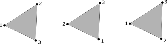
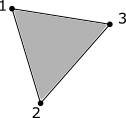
An orientation of a $k$-simplex $K$ is an ordering of the $0$-simplexes in $K$, written as $(v_0,…,v_k)$. We say that two orientations are the same if they differ by an even permutation. This means that any $k$-simplex for $k > 0$ has exactly two orientations. A $0$-simplex has only one orientation.

In the image below, the first two orientations on the $2$-simplex are considered the same, while, the third is not.

Simplicial Complexes

A simplicial complex is, roughly, a collection of simplexes that have been “glued together” in way that follows a few rules. A simplicial complex $K$ is a set of simplexes that satisfies

1. Any face of $K$ is also in $K$
2. The intersection of any two simplexes $\sigma_{1},\sigma_{2}\in K$ is a face of both $\sigma_{1}$ and $\sigma_{2}$.

Intuitively, we can think of building $K$ by iteratively glueing a face of a $k$-simplex to a $k-1$-simplex. So a $1$-simplex can be glued to a $0$-simplex at one–or both– of its endpoints, a $2$-simplex can be glued to a $1$-simplex along one of its edges, and so on.

We define an orientation of a simplicial complex $S$ to be an ordering of the $0$-simplexes contained in $S$. Two orientations are considered the same if they differ by an even permutation. Then each simplex in $S$ inherits an orientation from the orientation given on $S$.

Chains

The $k$-chains on a simplicial complex are a way of collecting all of the $k$-simplexes in a simplicial complex in an algebraic way. For an oriented simplicial complex $S$, we will write $S_k$ for all the oriented $k$-simplexes in $S$, where the orientation is inhereted from the orientation on $S$. Then the $k$-chains on $S$ will be denoted by $C_k$, and are all formal finite linear combinations of the form

where $c_i \in \mathbb{Z}$ and $\sigma_i \in S_k$, and $N = |S_k|$. We impose the condition that each oriented simplex is equal to the negative of the simplex formed with the opposite orientation. For example, if $\sigma = [v_1, v_2]$ is a $1$-simplex in $S$, where $v_1$ and $v_2$ are $0$-simplexes in $S$, then $-\sigma = [v_2, v_1]$ as an element of $C_k$.

With this notation, $C_k$ forms an abelian group with addition operation given by

The zero element of $C_k$ is given by the formal linear combination with $c_i = 0$ for all $i$.

Example

For the simplicial complex above, $3\cdot[1] + 5\cdot[2] - 2\cdot[3]$ is an element of $C_0$, and

is an element of $C_1$.

Boundary Maps

It turns out there are maps $\partial_k: C_{k} \rightarrow C_{k-1}$, which send a simplex to a linear combination of its faces. These maps turn out to be very useful.

If $\sigma = [v_0,…,v_k]$ is an orented $k$-simplex, we can define

where the oriented $k$-1 simplex

is the face of $(v_0,…,v_k)$ not containing the $0$-simplex $v_i$. Then $\partial_k$ is extended to $C_k$ by

Example

For the simplicial complex above, $\partial_1([1, 2]) = [2] - [1]$, and

Boundary Map Matrices

We can write the map $\partial_k$ as a matrix where the rows are indexed by the $k-1$ simplexes and the columns are indexed by the $k$-cycles.

Example

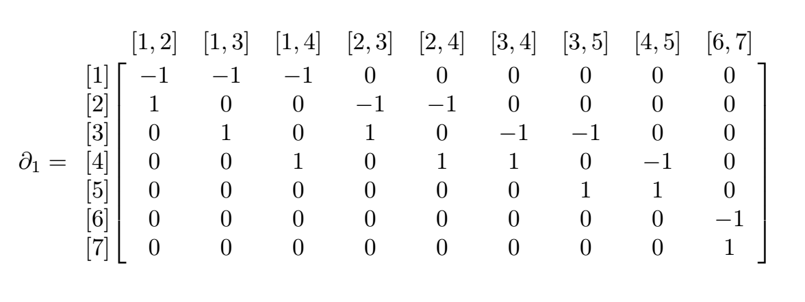
For the simplicial complex above, we can represent the map $\partial_1$ as the matrix

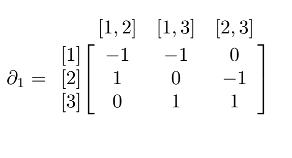
Now looking at our previous example, we can represent the element $11\cdot[1, 2] - 3\cdot[2,3]$ of $C_1$ as

and the previous calculation can be performed as the following matrix multiplication

Chain Complexes

These maps give what is called a chain complex:

One important relation for a chain complex is that

for all $k$. We will interpret this a bit more below.

Boundaries and Cycles

The elements of the image of the map $\partial_k$ in $C_{k-1}$ are called $k$-boundaries. We will write $Im(\partial_k)$ for the image of $\partial_k$.

Example

For the simplicial complex above, we have

as an element of $C_1$. Thus the element $[2, 3] - [1, 3] + [2, 3]$ is a $2-boundary$.

The elements of $C_k$ that are sent to zero in $C_{k-1}$ are called the $k$-cycles, and will be denoted $Ker(\partial_k)$. That is,

Example

For the simplicial complex above, we have

as an element of $C_0$, so $[1, 2] + [2, 3] - [1, 3]$ is a $1$-cycle. Notice that in this simplicial complex, this element is a cycle but not a boundary, since there are no $2$-simplexes in the simplicial complex.

Both $Im(\partial_{k+1})$ and $Ker(\partial_k)$ are subgroups of the group $C_k$. We can see now that the condition $\partial_{k+1} \circ \partial_k = 0$ means exactly that $Im(\partial_{k+1}) \subseteq Ker(\partial_k)$.

Homology

For an oriented simplicial complex $S$, we can now define the $k^{th}$ homology group as the quotient group

Informally, $H_k(S)$ is the group of $k$-cycles of $S$ “up to” any $k+1$-boundaries of $S$. That is, any $k+1$-boundaries in the group of $k$-cycles are treated as zero. For those that are familiar, this is analogous to modular arithmetic. For instance, arithemtic modulo $5$ treats $5$ the same as $0$, and so $\mathbb{Z}/5$ is the integers “up to” any multiple of $5: 17 = 2 + 3*5 \equiv 2 + 3*0 (mod5) = 2.$

Intuitively, we think of $H_k(S)$ as the $k$-dimensional holes in the simplicial complex $S$. So $H_0(S)$ will describe the number of connected components of $S$, $H_1(S)$ with describe the pieces of $S$ that look like circles, and $H_2(S)$ will describe the parts of $S$ that look like a hollow sphere, and so on.

Example

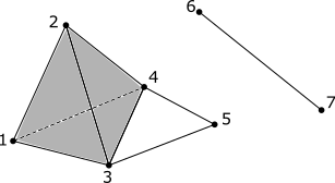
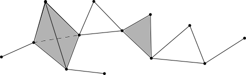
Let’s compute $H_0, H_1$ and $H_2$ of the above simplicial complex; let’s call it $S$. First, note that the part of the simplicial complex with vertices $1, 2, 3, \text{and } 4$ is hollow; not filled in; i.e. not a $3$-simplex.

$H_0(S)$ should count the connected components of $S$, which is $2$; let’s see how. Here is the relevant portion of the chain complex:

First, notice that since $\partial_0$ is the zero map, $Ker(\partial_0) = C_0$, so $H_0(S) = C_0/Im(\partial_1)$. Now let us see what $Im(\partial_1)$ is:

Now we can see that

Thus, in $C_1$, we have $[6] \equiv [7]$. In a similar fashion, we can see that

For example,

Thus the two unique elements of $H_0(S)$ are represented by $[1]$ and $[6]$, reflecting two connected components of $S$.

$H_1(S)$ should count the $1$-dimensional holes in $S$, which is $1$; let’s see how. Here is the relevant portion of the chain complex:

First, let us list out all elements $\sigma \in C_1$ such that $ \partial_1(\sigma) = 0$:

These are all the cycles in $C_1$; that is, they generate $Ker(\partial_1)$. Now let’s list the elements of $Im(\partial_2)$:

Now we can see that since the only element of $Ker(\partial_1)$ that is not in $Im(\partial_2)$ is $[3, 4] + [4, 5] - [4, 5]$, we can see that $H_1(S)$ is the group represented by integer multiples of this single element, indicating that there is a single $1$-dimensional hole in $S$.

Finally, $H_2(S)$ should count the $2$-dimensional holes in $S$, which is $1$; let’s see how. Here is the relevant portion of the chain complex:

Here, since there are no $3$-simplexes in $S$, $C_3 = 0$, and $Im(\partial_3) = 0$. Thus $H_2(S) = Ker(\partial_2)$. So let’s find what elements in $C_2$ map to $0$:

We can see that this only multiples of this element are sent to zero by $\partial_2$. So $Ker(\partial_2) = H_2(S)$ is generated by this single element; thus representing a single $2$-dimensional hole in $S$.

In the next section we will go over a more algorithmic way to calculate the homology groups. Hopefully this section, although lengthy, has shed some light on what is going on and why the $k^{th}$ homology group represents the number of $k$-dimensional holes in the simplicial complex. In fact, there is a little bit more going on than just counting; we will get into that a little below.

Calculating Homology using Smith Normal Form

For any $n\times m$ matrix $A$, there exist an invertible $n\times n$ matrix $U$ and an invertible $m\times m$ matrix $V$ such that $UAV$ is equal to a matrix of the form

Furthermore, if $A$ is an integer matrix, then $U, V$, and $D$ are all integer matrices, and the $\alpha_i$ satisfy $\alpha_{i}\mid \alpha_{i+1} \hspace{5pt} \text{for all} \hspace{5pt} 1 \leq i<r$. From this decomposition, we can see that $rank(A) = r$. Now we write down a result that will tell us how to compute homology groups; we do not give the proof, but if you wish, you can find it here.

${\bf Proposition.}$ Let $A$ be an $m\times n$ integer matrix, and $B$ be an $l\times m$ integer matrix such that $BA = 0$. Then

Where $r = rank(A)$, $s = rank(B)$, and $\alpha_1,…,\alpha_r$ are the non-zero elements on the diagonal of the Smith normal form of $A$.

Now we can see that if we take the matrix representations of $\partial_k$ and $\partial_{k+1}$ we can compute the $k^{th}$ homology group $H_k$ using the above proposition.

The portion of $H_k$ that is given by $\bigoplus_{i=1}^r \mathbb{Z}/\alpha_i$ is called the torsion part of $H_k$. The rank of $H_k$ is defined to be $m-r-s$ for $m$, $r$, and $s$ in the proposition above. The rank of $H_k$ is denoted by $\beta_k$, and is called the $k^{th}$ Betti number of the simplicial complex.

Example Let’s use our example simplicial complex from before to compute using Smith normal form. We will only compute $H_0(S)$ as the others are so similar as to not be helpful going through all of them.

To compute $H_0(S)$, first note that $ \partial_0 $ is the zero map, so its matrix representation is the $1 \times 7$ matrix of all zeros, and thus has rank $0$, and $Ker(\partial_0) = \mathbb{Z}^{|C_0|} = \mathbb{Z}^7$. Now let’s write down the matrix form of $\partial_1$:

We will not go into how to compute the Smith normal form here, but simply give the decomposition of this matrix:

where

In the formulation of Smith normal form above, $\partial_1 = A$, $U = W^T$, and $V=T^T$. From here we can compute the $H_0(S)$. Since $\mathbb{Z}/1 = 0$, $rank(\partial_0) = 0$, and $rank(\partial_1) = rank(D) = 5$, we have that

This lines up with our earlier computation of $H_0(S)$.

Example

This last example is of the Klein Bottle. It won’t be much as an example as an exercise. It is one whose $1^{st}$ homology group has torsion; i.e. it is not just copies of the integers. Below is a depiction of a simplicial complex structure for the Klein bottle. Let’s call this $K$. Here all the triangles are filled-in $2$-cells.

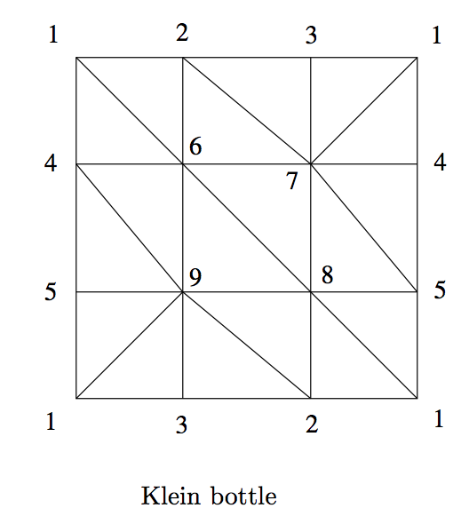
The above image is taken from the pdf of this project. The upshot will be that the first homology group of the Klein bottle will be

Below is python code taken from here to compute the Smith normal form of a matrix

from sympy import *

def leftmult2(m, i0, i1, a, b, c, d):
    for j in range(m.cols):
        x, y = m[i0, j], m[i1, j]
        m[i0, j] = a * x + b * y
        m[i1, j] = c * x + d * y

def rightmult2(m, j0, j1, a, b, c, d):
    for i in range(m.rows):
        x, y = m[i, j0], m[i, j1]
        m[i, j0] = a * x + c * y
        m[i, j1] = b * x + d * y

def smith(m, domain=ZZ):
    m = Matrix(m)
    s = eye(m.rows)
    t = eye(m.cols)
    last_j = -1
    for i in range(m.rows):
        for j in range(last_j+1, m.cols):
            if not m.col(j).is_zero:
                break
        else:
            break
        if m[i,j] == 0:
            for ii in range(m.rows):
                if m[ii,j] != 0:
                    break
            leftmult2(m, i, ii, 0, 1, 1, 0)
            rightmult2(s, i, ii, 0, 1, 1, 0)
        rightmult2(m, j, i, 0, 1, 1, 0)
        leftmult2(t, j, i, 0, 1, 1, 0)
        j = i
        upd = True
        while upd:
            upd = False
            for ii in range(i+1, m.rows):
                if m[ii, j] == 0:
                    continue
                upd = True
                if domain.rem(m[ii, j], m[i, j]) != 0:
                    coef1, coef2, g = domain.gcdex(m[i,j], m[ii, j])
                    coef3 = domain.quo(m[ii, j], g)
                    coef4 = domain.quo(m[i, j], g)
                    leftmult2(m, i, ii, coef1, coef2, -coef3, coef4)
                    rightmult2(s, i, ii, coef4, -coef2, coef3, coef1)
                coef5 = domain.quo(m[ii, j], m[i, j])
                leftmult2(m, i, ii, 1, 0, -coef5, 1)
                rightmult2(s, i, ii, 1, 0, coef5, 1)
            for jj in range(j+1, m.cols):
                if m[i, jj] == 0:
                    continue
                upd = True
                if domain.rem(m[i, jj], m[i, j]) != 0:
                    coef1, coef2, g = domain.gcdex(m[i,j], m[i, jj])
                    coef3 = domain.quo(m[i, jj], g)
                    coef4 = domain.quo(m[i, j], g)
                    rightmult2(m, j, jj, coef1, -coef3, coef2, coef4)
                    leftmult2(t, j, jj, coef4, coef3, -coef2, coef1)
                coef5 = domain.quo(m[i, jj], m[i, j])
                rightmult2(m, j, jj, 1, -coef5, 0, 1)
                leftmult2(t, j, jj, 1, coef5, 0, 1)
        last_j = j
    for i1 in range(min(m.rows, m.cols)):
        for i0 in reversed(range(i1)):
            coef1, coef2, g = domain.gcdex(m[i0, i0], m[i1,i1])
            if g == 0:
                continue
            coef3 = domain.quo(m[i1, i1], g)
            coef4 = domain.quo(m[i0, i0], g)
            leftmult2(m, i0, i1, 1, coef2, coef3, coef2*coef3-1)
            rightmult2(s, i0, i1, 1-coef2*coef3, coef2, coef3, -1)
            rightmult2(m, i0, i1, coef1, 1-coef1*coef4, 1, -coef4)
            leftmult2(t, i0, i1, coef4, 1-coef1*coef4, 1, -coef1)
    return (s, m, t)

m = Matrix([
    [-1, -1, -1, 0, 0, 0, 0, 0, 0],
    [1, 0, 0, -1, -1, 0, 0, 0, 0],
    [0, 1, 0, 1, 0, -1, -1, 0, 0],
    [0, 0, 1, 0, 1, 1, 0, -1, 0],
    [0, 0, 0, 0, 0, 0, 1, 1, 0],
    [0, 0, 0, 0, 0, 0, 0, 0, -1],
    [0, 0, 0, 0, 0, 0, 0, 0, 1]
    ])

smith(m)

Conclusion

We have seen the construction of homology groups, learned a bit about their interpretation and utility for studying topological spaces. We have also seen examples and methods for algorithmic computation of the homology groups given a simplicial complex structure, as well as some sample code you can use to get your feet wet with computing homology yourself!